
Executive summary
We trained a biological neural network built around a fruit fly’s wiring diagram to detect pleural effusion on chest X-rays, achieving 82% validation AUROC.
Introduction
In September 2026, researchers from HHMI Janelia, the University of Cambridge, the MRC Laboratory of Molecular Biology and Google Research published the MaleCNS connectome: a reconstruction of the adult male Drosophila melanogaster brain and ventral nerve cord containing more than 166,000 neurons [1, 2].
A connectome is a wiring diagram that tells us which reconstructed neurons connect to which others, how many synaptic contacts contribute to those connections, and properties such as predicted neurotransmitter identity.
We asked whether a network constrained by that wiring could learn to classify pleural effusion on chest X-rays. An image is sampled directly at R1–R6 photoreceptors, propagated through the complete MaleCNS graph, and classified from the resulting neural state. There is no learned image encoder before the connectome.
Visual input
Image preprocessing
We used frontal MIMIC-CXR radiographs [3, 4] with pleural effusion labels extracted from reports by CheXbert [5]. Each 512 × 512 image is converted to grayscale, resized without cropping, and padded to 224 × 224. For the prepared 8-bit pixel array , intensity at row and column is
These display intensities enter the model directly, without contrast equalization or a learned image encoder.
Retinal mapping
Of 3,377 annotated R1–R6 photoreceptors, 3,335 receive image coordinates; the other 42 remain in the graph without direct image input.
To locate receptor , we sum its contacts onto same-eye L1, L2 and L3 neurons by optic-lobe column . Let count contacts from source neuron to target neuron . The assigned column is
Ties are resolved by axial-coordinate order. The column's hexagonal coordinates become planar coordinates :
Using the minimum and maximum mapped coordinates within each eye, we normalize to :
Values are bounded to . The eyes occupy overlapping image viewports, with horizontal coordinate and vertical coordinate :
This inferred projection is not necessarily a calibrated model of fly optics. The 3,335 receptors occupy 824 distinct image positions .
Photoreceptor sampling
Bilinear interpolation gives each receptor one intensity. On the 224 × 224 canvas, its pixel coordinates are
Let and be the lower integer coordinates, with fractional offsets and . The sampled value is
The weights sum to one; some vanish at integer or boundary coordinates. Equivalently, expresses the sampling position on a coordinate system. Receptors at the same position receive the same value; there is no scanning or additional pooling.
Let identify receptor in the graph. The input vector places each sample at its corresponding neuron:
The dimensionless drive has gain 1 and stays constant through all twenty updates for an image. Neural state resets to zero for the next image.
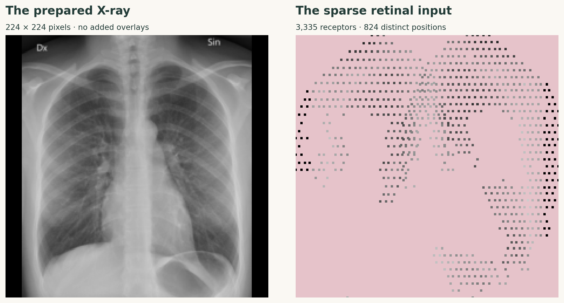
Figure 1. Photoreceptor sampling. Prepared radiograph and sampled intensities at their image locations; pink marks pixels that do not directly affect any receptor. This depicts the input mapping, not reconstructed or subjective fly vision. The demonstration image is by Mikael Häggström, CC0. It is not a MIMIC patient image.
_chest_radiograph_(X-ray).jpg)
Connectome model
Anatomical connectivity
The network contains neurons and 25,582,938 directed neuron-pair edges. Its fixed anatomical matrix is
Here is the contact count and the source neuron's sign. The sum over counts all incoming unsigned contacts to target ; absent connections remain zero. For predicted neurotransmitter ,
Unknown and other annotations take the positive branch. Each source has one sign across all outgoing connections, and is not learned.
Neural dynamics
Each neuron has learned latent parameters and , initially zero. They determine outgoing gain and leak :
Here is the logistic sigmoid and the hyperbolic tangent. Gains start at 1 and remain between 0.25 and 4; leaks start at 0.5 and remain between 0.05 and 0.95. These parameters are shared across all updates.
The effective connection is
Positive gains preserve the assigned signs and topology. All outgoing edges from neuron share , rather than receiving independent learned weights.
Starting from neural state , the model performs twenty synchronous updates:
Here is neuron 's state at step , and its image drive. Every neuron uses the previous state. In vector form, with denoting elementwise multiplication,
The states are signed, continuous, rate-like activations.
Classification
The classifier reads 148,763 neurons, excluding those annotated as sensory. Missing annotations are retained. The readout includes early visual interneurons but none of the directly driven receptors.
Let be this index set and . For each image, the final states become normalized features :
The term stabilizes the root-mean-square denominator; also scales for population size. No batch or cohort statistics enter this normalization.
Learned weights and bias produce logit and predicted pleural effusion probability :
Weights begin as independent normal draws with mean 0 and standard deviation 0.01; the bias begins at zero. Unlike anatomical gains, these artificial classifier parameters are unconstrained in sign.
The complete parameter set is
This counts all allocated parameters, including those of neurons that receive no input.
Training objective
The training set contains 7,859 positive and 13,396 negative images. Their ratio sets positive-class weight :
For a minibatch of images, label and logit give weighted binary cross-entropy
The loss averages over images. The same is used for validation. Gradients pass through all twenty updates, while the anatomical matrix stays fixed.
We used AdamW [6] with learning rates for and for , momentum coefficients , numerical stabilizer , and decoupled weight decay on all trainable parameters. Gradients were clipped to global L2 norm 5 before each update. Batch size was 64, retaining the final partial batch; initialization used seed 17.
Results
The model achieved 0.8241 validation AUROC and 0.6463 weighted validation cross-entropy at epoch 195.
- Validation AUROC
- 0.8241Epoch 195
- Training images
- 21,255Eligible images in the prepared cohort
- Recurrent updates
- 20Original sparse R1–R6 input
Only explicitly present or absent report labels were included; uncertain or unmentioned findings were excluded. Contradictory studies and identical images crossing partitions were removed. The partitions are patient-disjoint subsets of MIMIC-CXR:
| Partition | Images | Patients |
|---|---|---|
| Training | 21,255 | 6,729 |
| Validation | 3,774 | 1,194 |
We report results from the epoch with the highest validation AUC.
| Metric | Validation |
|---|---|
| AUROC | 0.8241 |
| Average precision | 0.6882 |
| Weighted binary cross-entropy | 0.6463 |
| Accuracy at probability 0.5 | 0.7530 |
| Balanced accuracy at 0.5 | 0.7554 |
| Sensitivity at 0.5 | 0.7630 |
| Specificity at 0.5 | 0.7478 |
AUROC measures ranking of positive versus negative images; average precision summarizes precision–recall ranking and depends on prevalence. Thresholded metrics use probability 0.5.
Figure 2. Validation performance across training. AUC and weighted binary cross-entropy on all 3,774 validation images, evaluated every five epochs. Points are measurements; lines connect them without smoothing. The two panels have separate vertical scales.
Discussion
The model learned to distinguish report-labelled pleural effusion while keeping the retinal mapping, anatomical topology and assigned synaptic signs fixed. Learning adjusted per-neuron gains and leaks, plus the artificial readout.
A fruit fly’s connectome is an unusual starting point for an X-ray classifier, but it proved a workable one. It also gives us a concrete way to explore how biological wiring shapes learning on a new task. A rather unexpected day job for a fly’s neural circuitry.
References
- Berg, S., Beckett, I. R., Costa, M., et al. “Sexual dimorphism in the complete Drosophila male central nervous system connectome.” Cell, 189(18), 5504–5526.e15 (2026). MaleCNS dataset.
- Januszewski, M., & Jain, V. “A connectomics milestone: Mapping the complete male fruit fly brain.” Google Research, September 3, 2026.
- Johnson, A. E. W., Pollard, T. J., Berkowitz, S. J., et al. “MIMIC-CXR, a de-identified publicly available database of chest radiographs with free-text reports.” Scientific Data, 6, 317 (2019).
- Johnson, A., Lungren, M., Peng, Y., Lu, Z., Mark, R., Berkowitz, S., & Horng, S. “MIMIC-CXR-JPG — chest radiographs with structured labels.” PhysioNet, version 2.1.0 (2024). Credentialed access conditions apply.
- Smit, A., Jain, S., Rajpurkar, P., Pareek, A., Ng, A., & Lungren, M. “Combining Automatic Labelers and Expert Annotations for Accurate Radiology Report Labeling Using BERT.” Proceedings of the 2020 Conference on Empirical Methods in Natural Language Processing, 1500–1519 (2020).
- Loshchilov, I., & Hutter, F. “Decoupled Weight Decay Regularization.” International Conference on Learning Representations (2019).